Note for the course Discrete-Time System Analysis.
1.1 Introduction
1.2 Discrete-Time Signals
Discrete-time Variable
If the time variable $t$only takes on discrete values $t=t_{n}$for some range of integer values of$n$, then$t$ is called discrete-time variable.
Discrete-time Signal
If a continuous-time signal $x(t)$is a function of discrete-time variable $t_{n}$, then the signal $x(t_{n})$ is a discrete-time signal, which is called the sampled version of the continuous-time function$x(t)$.
If we let $t_{n}=nT$, then obviously $T$is the sampling interval. When $T$is a constant, such a sampling process is called uniform sampling, instead, nonuniform sampling. Then we could write$x(t_{n})$ in form of$ x[n]$, in which square brackets is needed. And also,$x[n] = x(t_{n}) = x(t)|_{t=nT}=x(nT)$ .
Some typical examples of discrete-time signals
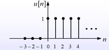
Discrete-Time Unit-Step Function
$$ u[n] = \left{\begin{matrix} 1,n=0,1,2, \cdots \ 0,n=-1,-2,-3,\cdots \end{matrix}\right. $$
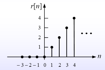
Discrete-Time Unit-Ramp Function
$$ r[n]=nu[n]=\left{\begin{matrix} n, n=0,1,2,\cdots \ 0,n=-1,-2,-3,\cdots \end{matrix}\right. $$
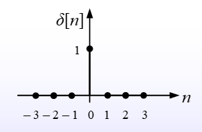
Unit Pulse
$$ \delta[n] = \left{\begin{matrix} 1,n=0 \ 0,n \neq 0 \end{matrix}\right. $$
Periodic Discrete-Time Signals
For a discrete-time signal $x[n]$, if there exists a positive integer $r$which makes that $x[n+r]=x[n]$for all integers n, Then $x[n]$ is called a periodic discrete-time signal and the integer$r$ is period. Fundamental period is the smallest value for positive integer$r$.
For example, if we let $x[n]=A\mathrm{cos}(\Omega n + \theta)$, then the signal is periodic if $x[n+r]=A\mathrm{cos}(\Omega (n + r)+\theta) = A\mathrm{cos}(\Omega n+\theta)$ .
Cause $\mathrm{cos}$is periodic, there is $A\mathrm{cos}(\Omega n + \theta) = A\mathrm{cos}(\Omega n + 2 \pi q + \theta)$ for all integers$q$ .
Obviously, $x[n]$is periodic when there exists an integer $r$which makes $\Omega r = 2 \pi q$for some integers$q$, in equivalent, the discrete-time frequency$\Omega = \dfrac{2 \pi q}{r}$ for some integers$q,r$.
Discrete-Time Complex Exponential Signals
$$ x[n]=Ca^{n}=|C||a|^{n}\mathrm{cos}(\omega _{0}n+\theta)+j|C||a|^{n}\mathrm{sin}(\omega _{0}n + \theta) $$
where $C = |C|e^{j\theta}$and$a = |a|e^{j\omega _{0}}$ .
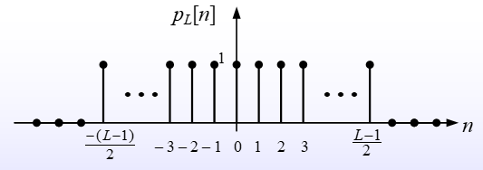
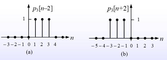
Discrete-Time Rectangular Pulse
$$ p_{L}[n] = \left{\begin{matrix} 1,;n=-\dfrac{L-1}{2},\cdots,-1,0,1,\cdots,\dfrac{L-1}{2} \ 0,; \mathrm{others} \end{matrix}\right. $$
where $L$ is a positive odd integer.
Digital Signals
When a discrete-time signal $x[n]$satiesfies that its values are all belongs to a finite set$\left{ a_{1},a_{2},\cdots,a_{n} }\right.$ , then the signal called a digital signal.
However, the sampled signals don’t have to be digital signals. For example, the sampled unit-ramp function values on a infinite set $\left{ 0,1,2,\cdots }\right.$.
Binary Signal is a digital signal whose values are all belongs in to set $\left{ 0,1 }\right.$.
Time-Shifted Signals
Giving a discrete-time signal $x[n]$and a positive integer$q$ , then
- $x[n-q]$is the $q$-step right shifts of$x[n]$
- $x[n + q]$is the $q$-step left shifts of$x[n]$
Discrete-Time Signals defined Interval by Interval
Discrete-Time Signals also may be defined Interval by Interval. For example, $$ x[n]=\left{\begin{matrix} x_{1}[n],;n_{1}\leq n < n_{2} \ x_{2}[n],;n_{2} \leq n < n_{3} \ x_{3}[n], ; n \geq n_{3} \end{matrix}\right. $$ Cause the Unit-Step Function satisfies when $n \geq 0$, $u[n]=1$ , we can use it to write$x[n]$ in such a form $$ x[n]=x_{1}[n]\cdot(u[n-n_{1}]-u[n-n_{2}]) +x_{2}[n]\cdot(u[n-n_{2}] - u[n - n_{3}]) +x_{3}[n]\cdot u[n - n_{3}] \ = u[n - n_{1}]\cdot x_{1}[n] +u[n - n_{2}]\cdot(x_{2}[n] - x_{1}[n]) +u[n - n_{3}]\cdot(x_{3}[n] - x_{2}[n]) $$
1.3 Discrete-Time Systems
Definition of Discrete-Time Systems and Analysis
The Discrete-Time System is a system which transforms discrete-time inputs to discrete-time outputs.
The Discrete-Time System Analysis is a process to solve the discrete-time output with discrete-time inputs and discrete-time system.
For example. Consider the differential equation $\dfrac{dv(t)}{dt}+av(t)=bx(t)$, now we resolve time into discrete interval forms of length$\bigtriangleup$ , so the equation will become $$ \frac{v(n\bigtriangleup)-v((n-1)\bigtriangleup)}{\bigtriangleup}+av(n \bigtriangleup)=bx(n \bigtriangleup) $$ which equals to $$ \frac{v[n]-v[n-1]}{\bigtriangleup}+av[n]=bx[n] $$ and $$ v[n]-\frac{1}{1+a\bigtriangleup}v[n-1]=\frac{b\bigtriangleup}{1+a\bigtriangleup}x[n] $$
1.4 Basic Properties of Discrete-Time Systems
System with or without memory
Given a discrete-time system with input of $x[n]$and output with $y[n]$ , we call the system memoryless when$y[n]$ is only related to input at present time, otherwise we call it is the one with memory.
For example, $$ y[n] = \sum_{k=- \infty}^{n}x[k] $$ and $$ y[n] = x[n] + x[n - 1] $$ are systems with memory, and $$ y[n]=(2x[n] - x[n]^{2})^{2} $$ is an example of system in memoryless.
Causality
Given a discrete-time system with input of $x[n]$and output with $y[n]$ , we call the system causal when$y[n]$ is only related to input at present and past time, or we call it not causal.
For example, $$ y[n]=\sum_{k=-\infty}^{n}x[k] $$ is system in causality, but $$ y[n]=x[n-1]+x[n+1] $$ not because $x[n + 1]$ is input in future, and $$ y[n]=x[-n] $$ is also not because when $n$is negative, there is$-n > n$ .
Time Invariance
To a discrete-time system with input of $x[n]$and output of $y[n]$ , we call the system time invariant when a time shifts in the input signal results identical time shifts in the output signal. This is also to say, output$y[n]$ is not explicity related on the varaible of time.
For example, $$ y[n]=(n+1)x[n] $$ is not time invariant because $y[n]$has an explicit relationship with time variable$n$.
and, the system $$ y[n]=x[2n] $$ is also not time invariant, because any time shift in input will be compressed by factor 2.
As an example of system which is time invariant, $$ y[n]=10x[n] $$ which is obvious.
Linearity
A system is to be called a linear system when the input consists of a weighted sum of several signals, the output will also be a weighted sum of the responses of the system for each of those signals.
To make a proof of a system to be in linearity, we let $y_{1}[n]$is the response of the system to the input $x_{1}[n]$, and$y_{2}[n]$ is the response of the input$x_{2}[n]$ . The system is a linear system if and only if
Addivity Property
The response to $x_{1}[n]+x_{2}[n]$is$y_{1}[n]+y_{2}[n]$.
Homogeneity Property
The response to $ax_{1}[n]$is $ay_{1}[n]$, for$a$ is any complex constant.
It’s interesting to find that a system with a linear equation may not be a linear system.
For example, considering the system $y[n]=2x[n]+3$, it’s easy to find the system is not linear, because
For two inputs $x_{1}[n]$and$x_{2}[n]$, there are
$x_{1}[n] \rightarrow y_{1}[n]=2x_{1}[n]+3$
$x_{2}[n] \rightarrow y_{2}[n]=2x_{2}[n]+3$
However, the response to input $(x_{1}[n]+x_{2}[n])$ is
$y_{3}[n]=2(x_{1}[n] + x_{2}[n])+3 \neq y_{1}[n]+y_{2}[n]$.
Notice that $y[n]=3$when $x[n]=0$, it reminds us that the system violates the “zero-in/zero-out” property and the zero-input response of the system is$y_{0}[n]=3$.